8.7 The CarbonLite Retrofit Model – assumptions

1. The CarbonLite Retrofit model

As we have discussed, investment decisions, whether by individual householders, social landlords with large property portfolios, investors looking to invest in energy efficiency projects, or local or central governments looking at regional or national programmes, are based on financial analysis, commonly referred to as ‘investment appraisals’.

Here we share some detailed analysis, carried out for CarbonLite, based on the range of retrofit scenarios described in Lesson 8.1. These give a sense of the lifetime costs and savings that can be expected from undertaking whole-house retrofit of some representative UK house types. The modelling carried out here takes into account a number of real-life factors absent from the more familiar “this measure will save you so much per year” advice.

Note – for the purposes of this course, we have analysed the costings from the point of view of owner occupiers, where the client pays for the work, and then pays the energy bills thereafter.

The model allows us to model the outcomes of different retrofit (or non-retrofit) scenarios involving different building types and factors in:

• Capital expenditure, costs for on-going maintenance, consumables and renewal of components at the end of their lifetimes (where shorter than the ‘lifetime period’ being considered), as well as heating costs
• State of the art modelling (using PHPP and THERM) of the thermal performance of the building’ fabric before and after retrofit
• The impact of occupant behaviour/lifestyle, including ‘comfort take’, which is now accepted to be the norm in real-life retrofits, but ignored in SAP and RdSAP
• Current and future energy prices
• The impact of geographical location (altitude, latitude, and exposure)

2. Lifetime costs

CLR modelling calculates for the three house types the ‘lifetime costs’ of the houses without deep retrofit, and with deep retrofit over 20 or 60 years including:

• component replacement (e.g. windows, equipment etc.)
• maintenance (fabric and equipment)
• consumables (e.g. MVHR filters)
• heating costs

The 60 year period is a notional, ‘industry standard’ lifetime for a building, looking at all costs for that building retrofitted in say 2020 out to 2080. It represents timeframes typically related to very large public infrastructure projects such as heat and power generation and distribution as well as timeframes used for climate change adaptation and mitigation policy.

A 20 year period represents the lifetime of a typical loan, so out to 2040 in the same example.

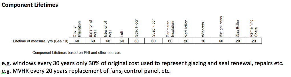
Individual components e.g. ventilation and heating systems, windows, roofing tiles, decorations etc. may have lifetimes less or more than the period over which the investment is being appraised. In the CLR modelling, the component lifetimes are based on ‘industry standard’ or Passivhaus Institute figures but can be changed as required for more bespoke modelling.

2.1 Life span of components

Retrofit components and measures, such as boilers, ventilation units and insulation-based fabric improvements all have their own specific life spans, varying from 10-60+ years, thus incurring replacement costs at regular intervals over the lifetime of the building.

As a result of retrofit measures some cyclical maintenance costs, such as repointing, redecorations related to mould staining, water ingress etc. might be reduced. If a retrofit measure ‘fails’ post retrofit, maintenance or repair costs might increase – underlining the importance of installing adequately robust measures!

CLR modelling uses a schedule of repair, maintenance and retrofit rates prepared by the CLR team and various contributors with a West Midlands Quantity Surveyor in 2014.

2.2 Lifetime

A lifetime period is chosen for an appraisal e.g. 60 years or 20 years in CLR examples. An average inflation rate over these periods is used (2%).

• The un-retrofitted basecase dwellings have a lifetime cost = heating fuel + maintenance + component replacement costs. This is the lifetime cost for each house type without retrofit.

• The retrofitted dwellings have a lifetime cost = (reduced) heating fuel + (reduced) maintenance + (ventilation) consumables + component replacement costs.

The lifetime marginal cost of a retrofit that forms the basis of the various ‘lifetime appraisal’ techniques discussed in this section = the ‘total lifetime cost of a retrofit’ – ‘total lifetime cost of its un-retrofitted basecase’.

The proportion of savings (reduced maintenance and lower heating bills) as a result of a moisture robust retrofit are obviously going to increase once any loan is paid off i.e. after the loan period, typically 20 years. This is why a business case appraised over a longer period (or at much lower borrowing interest rates) makes retrofit look more attractive.

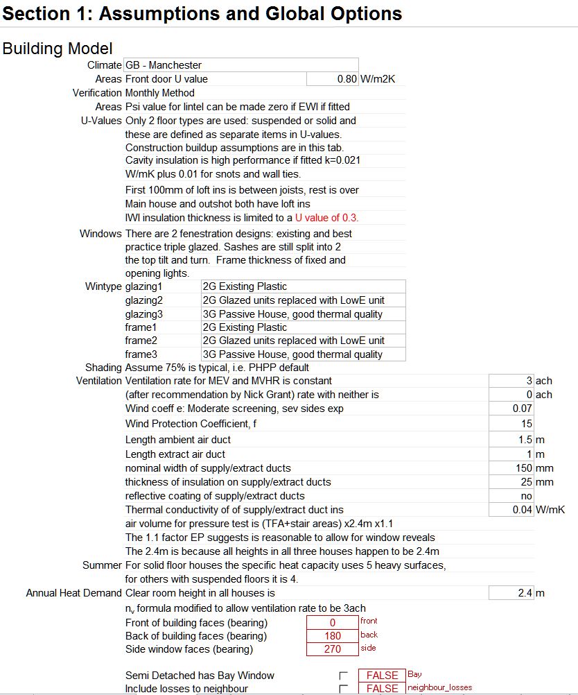
3. Relationship to PHPP

The CLR model is a non-commercial in-house customisation of the Passivhaus Planning Package (PHPP), and allows information input for a range of parameters

To give an idea of the level of detail, some parameters are illustrated below:

With any cost-benefit analysis it is essential to be explicit about the assumptions underlying the calculations – something often missing from reports based on simplistic costing methods.

The modelling tool developed for the CLR programme clearly records assumptions and allows them to be changed. This means we can create a large number of scenarios reflecting different financial conditions, different locations, or different building ownership or management patterns.

Obviously for this course the team have had to limit the number of scenarios used, and the scenarios used throughot the course material have been created to try to realistically illustrate energy and ecomomic performance before and after retrofit.

4. Parameters and values

For the illustrative scenarios used in this course we have created a fairly conservative current and future financial landscape. That is, one fairly harsh on deep retrofit in order to avoid over-optimistic thinking, to stress test the financial viability of deep retrofit and to build in some ‘slack’ for the effect of any errors and assumptions.

Through sensitivity testing – changing assumptions and parameters – we have identified the main factors that are likely to significantly change the economic attractiveness of deep retrofit, factors such as: policy incentives; including the value of co-benefits; financial incentives such as low cost finance; market maturation; and increased consumer recognition of and demand for energy efficiency.

Thus we have looked at a situation (excluding VAT) where there are:

• no grants
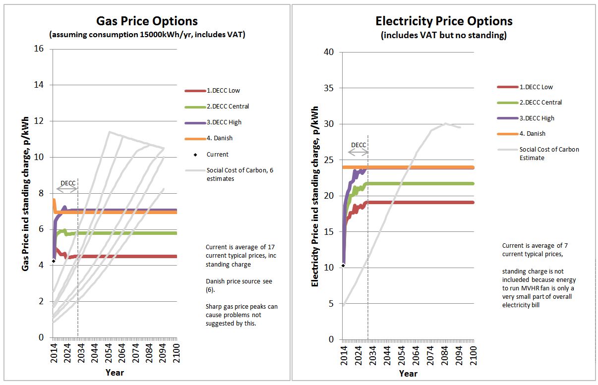
• only ‘modest’ increases in the price of energy (gas and electricity) assumed – specifically the ‘Central Scenario’ underlying The (as was) Department for Energy and Climate Change (DECC) official fuel cost forecasts.

There is an argument for assuming that fuel prices may not increase as much as the CLR scenario suggests, however we have not currently assumed this to be the case in our modelling.

The homes modelled are assumed to be heated by gas, as this is far and away the most common heating fuel in the UK. Despite talk of ‘weaning ourselves off gas’, natural piped gas, delivered through the national gas grid seems likely to continue to be a major heating-energy carrier for many years. The addition of biomethane is one example of future measures to decarbonise gas.

5. Co-benefits and ‘comfort take’

Consider occupants NOT increasing their room temperatures after investing in retrofit:

Even if ‘comfort take’ does not occur – retrofitting brings certain co-benefits.

There are some co-benefits of deep retrofit even without taking the 3°C rise in temperature because even without taking benefit in terms of increased room temperatures, a retrofit will result in improved comfort compared to the pre-retrofitted basecase. These benefits result from:

1. No draughts because airtightness is improved. Draughts and cold spots in an unimproved house can also be caused by indoor air being chilled next to poor glazing, and then circulating back into the room: this effect is reduced by medium retrofits (higher quality double glazing) and removed by deep ones (triple glazing)
2. Thermostat still set at ‘17°C’ but it feels warmer, not only because of reduced draughts but also by the higher radiant temperature of the surfaces surrounding occupants.

• Improved indoor air quality compared to the pre-retrofitted basecase because of the use of an effective ventilation system (e.g. MVHR or MEV)

Co-benefits of deep retrofit with a 3°C rise in temperature:

As long as the retrofit is comprehensive (i.e. is “deep” enough) an increase in house temperature becomes affordable, whilst at the same time maintaining the majority of the fuel savings. Too shallow a retrofit would mean that comfort take increases house temperatures but eats up all the fuel savings or even increases fuel use!.

• In a deeper retrofit the house can now be heated, for example, to 20°C (the default CLR assumption) or even 22°C without the bills rising precipitously as would have happened in the original unimproved house. This co-benefit has significant value particularly for: people working from home; older people (and also those who care for or about them); families with very young children; or for occupants in poor health.

Co-benefits of deep retrofit irrespective of the degree of comfort take:

• Deeper retrofits offer robust long-term protection against fuel poverty whilst allowing a good degree of flexibility for different lifestyles or changes in health.
• Minimum indoor temperatures during financial problems, fuel shortages or blackouts won’t fall as low in a deeper retrofit

Other co-benefits:

To occupants

• Future energy price rises have reduced impact (the more they rise, the more you save)
• House is cleaner and more pleasant, less housework!

To owners

• Value of house could be increased (although whether this is actually realised on sale is sensitive to market conditions)
• Maintenance (e.g. redecoration, replastering) should be reduced
• Reduced impact of fuel price inflation (capital invested in retrofit has been substituted for a significant portion of fuel costs)

In addition there will be benefits to the energy supply system and the country as identified in the discussion of co-benefits.

(We look elsewhere in this Module at the value of national level co-benefits.)

6. Borrowing rate

We have assumed a borrowing rate of 3.5% for financing the retrofit work, not the Green Deal borrowing rate (now defunct). This is close to current typical mortgage rates, and is also the rate to use for investment appraisals relating to public works set out in the Treasury Green Book. Depending on economic circumstances, Public Utilities can borrow at even lower rates for some infrastructure projects – although currently this may not be the case. Likewise Government (borrowing at the ‘Gilts rate’) can borrow at low rates for infrastructure projects – which is currently the case.

7. Assumptions for CLR illustrative material in this Module

Parameters included in the model and the values assumed for the main modelling exercise are noted below in brackets.

Building:
Location (Manchester).
Wind protection and sheltering coefficients affect the infiltration (mid-range) .
Orientation (houses modelled with front facing north)

Heating/behaviour:
Comfort taking (yes, 3°C)
Temperatures before and after (17°C before, 20°C after)
Heating fuel type (natural gas only)

Economic/financial:
Borrowing interest rates (3.5%, please pay attention to where the financial investment methods covered later in this module do or don’t included financing costs)
Inflation rate (2%)
Grants and/or use of personal savings (none)
Fuel Price Increase pattern above inflation (DECC’s ‘Central’ scenario):

The assumptions on inflation and fuel costs are perhaps the least certain of any because even past trends are no indication of future values. Therefore it is essential to examine the impact of a wide range of possible combinations to see where higher risks might lie.

NB: DECC scenarios are only forecast out to 2030 i.e. 15 years. Where CLR has used a 60 year time period we have simply extended a constant line after that to 60 years, which of course becomes an even more unreliable assumption.

Note that the grey lines relate to the social cost of carbon discussed in Lesson 8.3, as modelled by Stern and Dietz. The implication here is that current and future energy costs are not enough to stimulate a change consumption behaviour without other incentives.